Gradients and Surfaces

The R Language

I'm going to use the R language for all the graphics in this post since it is free, open source and runs on a variety of platforms (although they will need to support OpenGL. Macs come with this as standard). R is generally used for statistics but it will work in other areas of mathematics. Just don't be too pedantic as to how it does this…

Surfaces

Given a function:

f(x, y) = x^2 + y^2

(where the ^ symbol here uses the R-language notation for "to the power of"), we can generate the plot in the range for x and y of -5 to 5:

The R code for this is:

# load the graphics library
library(rgl)

# define our function
myFunc <- function(x, y)  x ^ 2 + y ^ 2

# Let's create a structure called 'data'
data.x     = seq(-5, 5, 1) # x is the open set from -5 to 5 in unit steps
data.y     = seq(-5, 5, 1) # ditto for y

# create a grid (in namespace 'data.xyz') that holds x and y
data.xyz   = expand.grid(x=data.x, y=data.y)
# in this same namespace, add 'z' which uses our function 
data.xyz$z = myFunc(data.xyz$x, data.xyz$y)

# some R graphics
nbcol = 100
# rev() means reverse. rainbow() gives us colours
color = rev(rainbow(nbcol, start = 0/6, end = 4/6))
# cut() breaks the data in z into nbcol units
zcol  = cut(data.xyz$z, nbcol)

# purely for convenience
mydata = data.xyz

plot3d(mydata $x, mydata$y, mydata$z, 
#aspect=FALSE, # scale with the window
xlab="x", ylab="y", zlab="z")

# spread a multi-coloured surface over these points
# note that data.x and data.y are just the unique values for x and y
# whereas data.xyz.$z is all the calculated points using x and y.
# Naturally, length(mydata.$z) = length(data.x) * length(data.y)
surface3d(data.x, data.y, mydata$z, col=color[zcol])

So, as far as our graph goes, the value on the z-axis is f(x, y). Equivalently, we can express this surface as the implicit function:

F(x, y, z) = 0 

since

z = f(x, y)

then we can say that for this surface:

F(x, y, z) = 0 = z - f(x, y) = f(x, y) - z

the order of f(x, y) and z in the above equation is significant when we calculate the normal to the surface (it determines whether it points in or out).

The gradient of this function gives us the normal to the surface (see this link for why).

Given:

then

div F = div( f(x, y) - z) = 2x i + 2y j - k

Putting this into our R script:

# c() is built-in R function to make vector-like objects
# matrix() makes matrix-like objects. This one makes a matrix
# of all the vector like collections of x, y and z objects in
# mydata. It has height 3 and a length equal the number
# of data points of x, y and z
mat=matrix(c(mydata$x, mydata$y, mydata$z ), 3, byrow=TRUE)

for (t in seq(1, length(mat)/3, 1)) { # /3 because we have 3 dimensions
dx   = 2 * mat[1,t]   # from the equation above
dy   = 2 * mat[2,t]   # from the equation above
dz   = -1             # from the equation above
from = mat[,t]        # vector of start point
to   = c(mat[1,t] + dx, mat[2,t] + dy, mat[3,t] + dz)
vec  = rbind(from, to)# list of the start and end point
segments3d(vec)       # that makes this line
}

and running it, we get to see the normals of our surface.

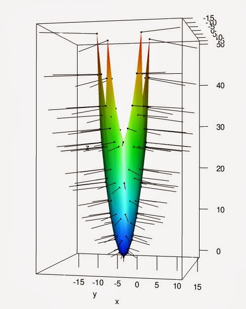
This time, I run the script with the aspect=FALSE uncommented as I want the scaling to be more representative.